Building a Data Pipeline in Python with Scikit-Learn and Pandas

Introduction

In data science, a data pipeline refers to the series of processes that are used to extract, transform, and load (ETL) data from its source to a destination, such as a database or a data warehouse. Building an efficient data pipeline is crucial for ensuring that the data is properly cleaned and preprocessed before it is used for analysis or modelling.

In this blog post, we will walk through an example of building a data pipeline in Python using the Scikit-Learn and Pandas libraries. Specifically, we will use Scikit-Learn's Pipeline class to create a pipeline that extracts data from a webpage, cleans and preprocesses it using Pandas, and finally outputs the processed data in a DataFrame.

Setting up the Environment

To get started, we first need to set up our environment with the necessary libraries. We'll need Pandas, Scikit-Learn, and requests for making web requests. You can install them by running the following commands in your terminal:

pip install pandas
pip install scikit-learn
pip install requests

Step 1: Extracting Data from a Webpage

Our data source for this example will be a webpage that contains a table of countries ranked by sex ratio. We'll use the requests library to make a web request to the page and extract the table using the BeautifulSoup library. Here's the code for the get_webpage_tables function:

import requests
from bs4 import BeautifulSoup

def get_webpage_tables(url):
    page = requests.get(url)
    soup = BeautifulSoup(page.content, 'html.parser')
    tables = soup.find_all('table')
    return tables

This function takes a URL as input and returns a list of all the tables on the page. We'll use this function as the first step in our data pipeline.

Step 2:Cleaning and Preprocessing the Data

Now that we have the table data, we need to clean and preprocess it. We'll use Pandas to do this. Specifically, we'll use Pandas to:

Select the table we want to use
Remove unnecessary rows and columns
Rename columns
Convert data types

Here's the code for the extract_country_sex_ratio function:

import pandas as pd

def extract_country_sex_ratio(tables):
    table = tables[0] # Select first table
    df = pd.read_html(str(table))[0] # Convert HTML table to DataFrame
    df = df.iloc[1:] # Remove first row
    df = df[['Country or territory', 'Male:female ratio']] # Select relevant columns
    df = df.rename(columns={'Country or territory': 'Country', 'Male:female ratio': 'Ratio'}) # Rename columns
    df['Ratio'] = pd.to_numeric(df['Ratio'], errors='coerce') # Convert Ratio column to float
    df = df.dropna() # Remove rows with missing values
    return df

This function takes the list of tables returned by the get_webpage_tables as input, selects the relevant table, and performs the cleaning and preprocessing steps described above. The output is a Pandas DataFrame containing the cleaned and preprocessed data.

Adding Country Codes

Finally, we'll add country codes to the DataFrame using a mapping table. Here's the code for the get_country_codes function:

def get_country_codes(df) ->  pd.DataFrame:
    """
    Retrieves ISO country codes from a GitHub repository and returns a cleaned DataFrame
    """
    country_raw = pd.read_csv('https://raw.githubusercontent.com/lukes/ISO-3166-Countries-with-Regional-Codes/master/all/all.csv')
    df_c = country_raw.iloc[:, [0,2]]
    df_c = df_c.rename(columns={'name':'Country', 'alpha-3':'ISO-code'})
    df_c = df_c.drop_duplicates(subset=['Country'], keep='last').dropna()

    # Manually modify some of the country names to match the names in the main DataFrame
    df_c.at[df_c[df_c['Country']=='Viet Nam'].index.values[0], 'Country'] = 'Vietnam'
    df_c.at[df_c[df_c['Country']=='United States of America'].index.values[0], 'Country'] = 'United States'
    df_c.at[df_c[df_c['Country']=='Iran (Islamic Republic of)'].index.values[0], 'Country'] = 'Iran'
    df_c.at[df_c[df_c['Country']=='Russian Federation'].index.values[0], 'Country'] = 'Russia'
    df_c.at[df_c[df_c['Country']=='United Kingdom of Great Britain and Northern Ireland'].index.values[0], 'Country'] = 'United Kingdom'
    df_c.at[df_c[df_c['Country']=='Venezuela (Bolivarian Republic of)'].index.values[0], 'Country'] = 'Venezuela'
    df_c.at[df_c[df_c['Country']=="Korea (Democratic People's Republic of)"].index.values[0], 'Country'] = 'Korea, North'
    df_c.at[ df_c[df_c['Country']=='Korea, Republic of'].index.values[0], 'Country' ] = 'Korea, South'
    df_c.at[ df_c[df_c['Country']=='Bolivia (Plurinational State of)'].index.values[0], 'Country' ] = 'Bolivia'
    df_c.at[ df_c[df_c['Country']=='Côte d\'Ivoire'].index.values[0], 'Country' ] = 'Ivory Coast'
    df_c.at[ df_c[df_c['Country']=='Congo'].index.values[0], 'Country' ] = 'Congo, Republic of the'
    df_c.at[ df_c[df_c['Country']=='Tanzania, United Republic of'].index.values[0], 'Country' ] = 'Tanzania'
    # Using the ISO-3166 coding standard to map countries
    df['ISO-code'] = df['Country'].map(df_c.set_index('Country')['ISO-code'])
    # Clean data-frame ( Duplicates & NaNs )
    df.isna().sum() 
    df = df.dropna()
    return df

Step 3: Defining the Pipeline

Now that we have our helper functions, we can define our pipeline. The pipeline is a series of steps that our data will go through in order to transform it into the desired format. In our case, we want to extract the country codes from the Wikipedia table.

We'll use the Pipeline class from the scikit-learn library to define our pipeline. This class allows us to define a series of steps that will be executed in order. In our case, we'll have three steps:

get_tables: This step will use the get_webpage_tables function to extract the tables from the Wikipedia page.
extract_ratio: This step will use the extract_country_sex_ratio function to extract the sex ratios for each country from the tables.
get_codes: This step will use the get_country_codes function to extract the country codes from the Wikipedia page.

We can define our pipeline like this:

from sklearn.pipeline import Pipeline
from sklearn.preprocessing import FunctionTransformer

# define pipeline
pipeline = Pipeline([
    ('get_tables', FunctionTransformer(get_webpage_tables)),
    ('extract_ratio', FunctionTransformer(extract_country_sex_ratio)),
    ('get_codes', FunctionTransformer(get_country_codes))
])

Each step is defined as a tuple with two elements. The first element is a string that represents the name of the step, and the second element is an instance of the FunctionTransformer class from scikit-learn. The FunctionTransformer class is used to wrap our helper functions so that they can be used as steps in the pipeline.

Step 4: Applying the Pipeline

Now that we have defined our pipeline, we can apply it to our input URL using the transform method. This method will apply each step of the pipeline to transform our input data into the desired format.

# apply pipeline to input URL
df = pipeline.transform(url)

df

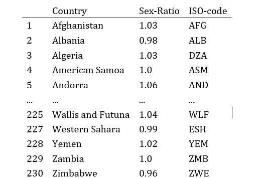
This will return a pandas DataFrame with the country codes and sex ratios for each country.

After running the pipeline, the resulting dataframe df contains the sex-ratio of each country, along with their ISO country codes. To visualize this data, we can use Plotly Express, a Python visualization library that allows us to create interactive and high-quality visualizations with just a few lines of code.

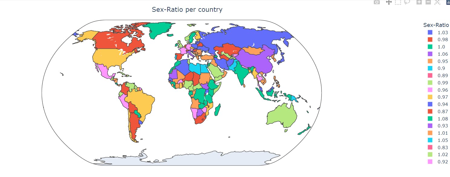
In the following code snippet, we set a threshold value of 1.3, and remove all countries with a sex-ratio greater than this value. Then we create a choropleth map using Plotly Express, where each country is colored according to its sex-ratio value. We use the ISO country codes to match each country to its corresponding geographic location on the map.

import plotly.express as px

thres = 1.3
df_th = df.drop(df[ df['Sex-Ratio'] > thres ].index)

# color pallete @ https://plotly.com/python/builtin-colorscales/
fig = px.choropleth(df_th, locations='ISO-code',
                color="Sex-Ratio", hover_name="Country",
                    color_continuous_scale=px.colors.sequential.Sunset, projection="natural earth")
fig.update_layout(title={'text':'Sex-Ratio per country', 'y':0.95, 'x':0.5, 'xanchor':'center', 'yanchor':'top'})
fig.show()

In the first line, we import the Plotly Express library using the px alias. We then set a threshold value of 1.3, above which countries are excluded. We create a new dataframe df_th by dropping all countries with a sex-ratio greater than this value.

Next, we use Plotly Express to create a choropleth map using the px.choropleth() function. We pass df_th as the first argument, which contains the data we want to plot. We specify the locations argument as 'ISO-code', which tells Plotly Express to use the ISO country codes as the locations for each data point. We set the color argument to 'Sex-Ratio', which tells Plotly Express to color each data point according to its sex-ratio value. We also specify the hover_name argument as 'Country', which tells Plotly Express to display the name of each country when we hover over its corresponding data point.

We use the color_continuous_scale argument to specify the color palette we want to use for the map. In this case, we use the px.colors.sequential.Sunset color palette, which ranges from blue to yellow to red. Finally, we set the projection argument to "natural earth", which tells Plotly Express to display the map using a natural Earth projection.

We then update the layout of the plot using the fig.update_layout() function. We set the title argument to a dictionary containing the title text, as well as the position and alignment of the title. Finally, we call the fig.show() function to display the plot in a new window or notebook cell.

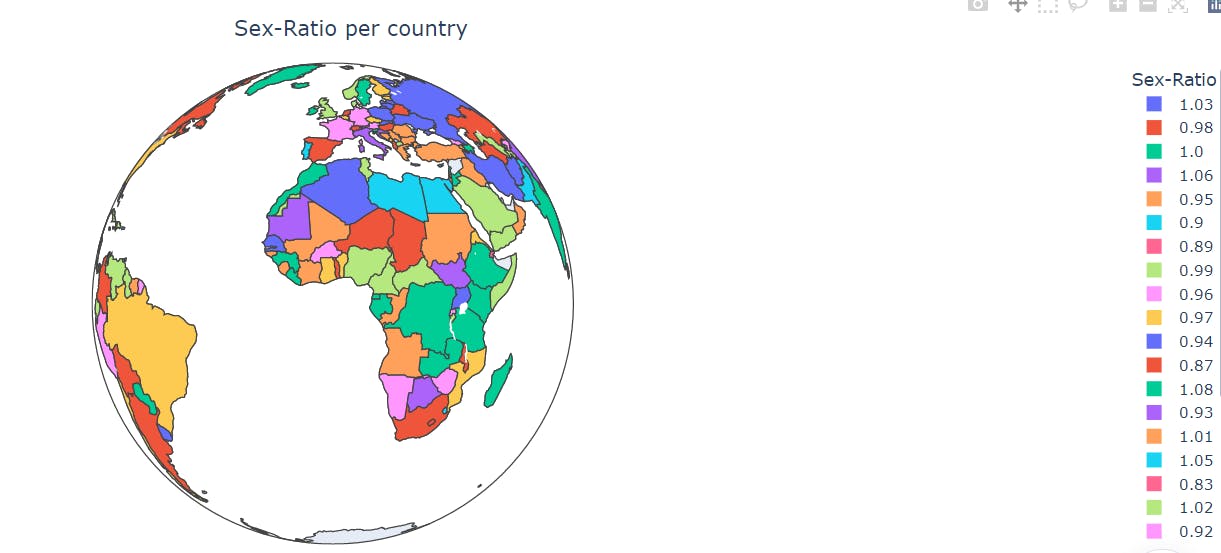
Below the plot from the code

This code creates a choropleth map using Plotly Express to visualize the sex ratio per country, but with a different projection.

geographic location on the map.

import plotly.express as px

thres = 1.3
df_th = df.drop(df[ df['Sex-Ratio'] > thres ].index)

# color pallete @ https://plotly.com/python/builtin-colorscales/
fig = px.choropleth(df_th, locations='ISO-code',
                color="Sex-Ratio", hover_name="Country",
                    color_continuous_scale=px.colors.sequential.Sunset, projection="orthographic")
fig.update_layout(title={'text':'Sex-Ratio per country', 'y':0.95, 'x':0.5, 'xanchor':'center', 'yanchor':'top'})
fig.show()

First, a threshold value of 1.3 is set to remove any countries with a sex ratio above this value. This is done using the drop() function and the index parameter, which removes the rows where the sex ratio is greater than the threshold.

Next, a choropleth map is created using the px.choropleth() function from Plotly Express. The df_th DataFrame is used as the data source, with the locations parameter set to the ISO-code column, the color parameter set to the Sex-Ratio column, and the hover_name parameter set to the Country column.

The color_continuous_scale parameter is set to px.colors.sequential.Sunset to define the color palette for the map. Finally, the projection parameter is set to "orthographic" to create a different projection for the map.

The fig.update_layout() function is used to add a title to the map, with the text, y, x, xanchor, and yanchor parameters specifying the text, vertical position, horizontal position, horizontal alignment, and vertical alignment of the title, respectively.

Finally, the fig.show() function is called to display the map.

Conclusion

In this blog post, we have demonstrated how to extract data from a Wikipedia page using Python and scikit-learn. We used the requests library to download the HTML source code of the Wikipedia page, and the BeautifulSoup library to extract the relevant tables. We then used a pipeline with scikit-learn to extract the sex ratios and country codes from the tables. The resulting data was then stored in a pandas DataFrame for further analysis.

I hope that this blog post has been helpful in demonstrating how to extract data from web pages using Python and scikit-learn. If you have any questions or comments, please feel free to leave them below!

BitsnBytesofAI